bayesloop - Probabilistic programming framework

features

In contrast to MCMC methods and the Variational Bayes approach, bayesloop uses a discrete, regular grid to represent parameter distributions.

Computing the model evidence for hypothesis testing then reduces to a simple sum over all lattice points on this grid!

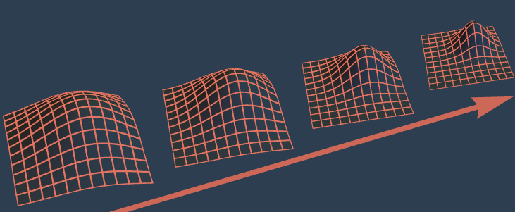
By inferring parameter distributions sequentially, time step by time step, bayesloop effectively breaks down one high-dimensional inference problem into many low-dimensional ones.

This efficient approach can be employed for both retrospective and online analyses!

bayesloop serves a specific niche of statistical models: We focus on well-known, simple statistical models with only few parameters, and extend these parameters to be time-varying.

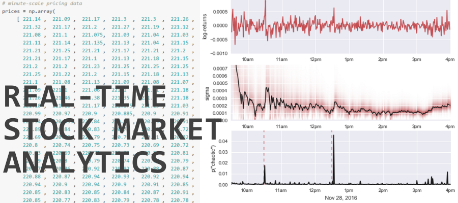
The resulting time-varying parameter models rest on a well-known statistical foundation and yet offer new insights into complex systems like invasive cancer cells or financial markets!

getting started

bayesloop is a Python module and the latest stable version is most easily added to your existing Python distribution via the built-in package manager:

pip install bayesloop

Alternatively, a zipped version can be downloaded here. In that case, the module is installed by calling

python setup.py install

Further information about the installation of bayesloop and troubleshooting can be found in the documentation.

minimal example

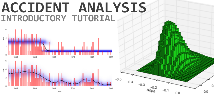
The following code provides a minimal example of an analysis carried out using bayesloop. The data here consists of the number of coal mining disasters in the UK per year from 1851 to 1962 (see this article for further information).

import bayesloop as bl
import matplotlib.pyplot as plt
import seaborn as sns

S = bl.HyperStudy()  # start new data study
S.loadExampleData()  # load data array

# observed number of disasters is modeled by Poisson distribution
L = bl.om.Poisson('rate')

# disaster rate itself may change gradually over time
T = bl.tm.GaussianRandomWalk('sigma', bl.cint(0, 1.0, 20), target='rate')

S.set(L, T)
S.fit()  # inference

# plot data together with inferred parameter evolution
plt.figure(figsize=(8, 3))

plt.subplot2grid((1, 3), (0, 0), colspan=2)
plt.xlim([1852, 1961])
plt.bar(S.rawTimestamps, S.rawData, align='center', facecolor='r', alpha=.5)
S.plot('rate')
plt.xlabel('year')

# plot hyper-parameter distribution
plt.subplot2grid((1, 3), (0, 2))
plt.xlim([0, 1])
S.plot('sigma', facecolor='g', alpha=0.7, lw=1, edgecolor='k')
plt.tight_layout()
plt.show()

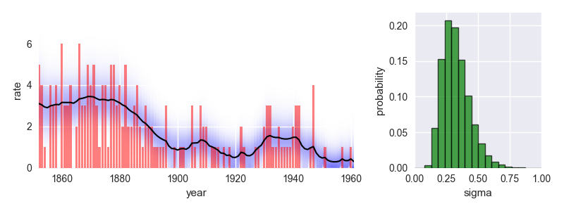
This analysis indicates a significant improvement of safety conditions between 1880 and 1900. Check out the documentation for further insights into this dataset!

The documentation further provides a detailed description of all features of bayesloop, including inference and hypothesis testing for time-varying parameter models, the detection of change-points and structural breaks in time series data, the prediction of future parameter values, the handling of missing data points, custom models based on the statistics modules of SymPy and SciPy, and model selection for online data streams.

Documentation